Getting Started in WebGL, Part 1: Introduction to Shaders

Shaders are at the heart of most graphics applications and APIs. Typically around half of your WebGL code will be about creating and interfacing with shaders. A good understanding of shaders is therefore necessary. In this tutorial, I’m going to show you around the graphics pipeline (the series of sequential operations performed on the inputs to produce the results), explain what shaders are and while at it we’ll write our first shader. Note: you don’t have to remember everything mentioned in this article. Only by extensive practice will it ever settle in. So, don’t take it too seriously. Enjoy reading it now, and you can always return to it for more details later.

What Are Shaders?

In graphics APIs, a shader is a computer program that is used to do shading: the production of appropriate levels of color within an image. It’s the right answer, but I bet you are not satisfied! For better understanding, we’ll quickly review the history of shaders to know what they are and what lead to them.

What Are Shaders?

At the beginning, there was software rendering. You’d typically have a set of functions that draw primitives, like lines, rectangles and polygons. By calling one of these functions the CPU would start rasterizing the primitive (filling the pixels that belong to it on the screen). How these primitives should look was either specified in function arguments or set in state variables. Later, it was clear that CPUs are not particularly efficient in doing graphics. They are general purpose by design, so they don’t make assumptions about the nature of the programs they are going to run. They provide large and diverse instruction sets to handle all kinds of things, like interfacing memory and I/O, interrupt handling, access protection, memory paging, context switching and a plethora of other stuff. Drawing graphics is just one of many things CPUs can do. And to make things worse, they have to do all these things virtually simultaneously. A solution had to be found to support the ambitions of graphics developers (ehm, and game developers). It was clear that better performance required more specialized hardware. Since 1975, hardware implementations of some of the computationally expensive graphics operations came to existence. Graphics workstations, arcades and game consoles were the first to adopt the new technologies. Personal computers were quite late to join the party. This gave a good boost in performance, but was just not enough. So, hardware manufacturers responded by implementing drawing primitives in hardware, relieving the CPU from this burden altogether. Professional solutions existed since the 1980s, but only in 1995 did 3DLabs release the first accelerated 3D graphics card aimed at the consumer market. Software rendering was still very popular back then, and games were among the most important reasons for users to upgrade their CPUs. CPU manufacturers had to maximize on this selling point. They had to come up with something to reinforce their gaming abilities. One of the core areas that were addressed was vector arithmetic. Graphics applications make heavy use of floating point vectors and matrices. Since 1997, hardware manufacturers started including multi-media targeted specialized instruction sets in their CPUs, like MMX, SSE and 3DNow!. These instructions were different to regular arithmetic instructions by being SIMD (Single Instruction Multiple Data). You could do vector operations in one go, like adding 4 values to another 4 values in one instruction instead of four. As awesome as they are, game developers demanded more! Games became more CPU demanding than ever. They needed better physics, better AI, better sound effects …etc. Even multi-core processors that came later couldn’t compete with separate hardware whose sole purpose is accelerating graphics. Advanced versions of the SIMD instruction sets still exist in modern CPUs, but are more commonly used in software rendering suites, video encoders/decoders and hardware emulation software.

The Fixed Pipeline

Graphics APIs filled the gap between the applications and the graphics hardware. They acted like an abstraction layer that hides the details of the hardware implementation, and provides a software implementation if hardware acceleration is not present. This made developers worry less about hardware compatibility. It was the responsibility of the hardware manufacturers to provide drivers that implement the popular APIs. It was up to the manufacturer to decide the API level the hardware is going to support, how much of it is going to be implemented in hardware, how much will be emulated in software (the driver) and how much won’t be supported at all. OpenGL and Glide were among the APIs with early support for consumer level hardware acceleration. Graphics APIs were not limited to drawing primitives only. They also did transformations, lighting, shadows and lots of other stuff. So, lets say you wanted to add a light source to your scene. The API gave you means of detecting the maximum number of lights supported by the hardware. You would then enable one of these lights, set its source type (point, spot, parallel), color, power, attenuation …etc. Finally the light is usable. Shadows? You’d have to set its bla bla bla. Anything else? Bla bla bla. It was inevitable that a certain way of doing things had to be forced to enable maximum compatibility. This was called the fixed pipeline. Although it’s customizable, it’s still fixed. Developers were limited by the API capabilities, which had to grow larger with every release.

Something to Be Desired

While it worked for games, an entirely fixed-pipeline is not very useful for scientific and cinematic graphics. These have to be more innovative and to break the mold quite often. Since 1984, some pioneers worked on “shaders”. Instead of performing a fixed function, the renderer would execute some arbitrary code to achieve the desired results. This was made possible in Pixar’s RenderMan around 1989, but only as a software implementation. Like almost every other technology, stuff that belongs to the labs take their time then become democratized. By the end of the 1990s, it was obvious that programmable graphics hardware was the right next step. For around a decade hardware manufacturers were shying from this, but they finally had to do it. Games were pushing the limits, and graphics APIs were becoming huge. It was time to stop telling developers what they can and can’t do and give them control over their hardware. Thus, pieces of the graphics pipeline were made programmable. Fragment processing (assume a fragment is a pixel for now) was the first to become programmable, followed by vertex processing. The first consumer graphics cards supporting both types of shaders hit the market in 2001. Later, the graphics pipeline became more flexible and allowed for more types of shaders to fit in. Now it’s up to the developers to decide how they want to process their data to produce their desired results. This opened the door for limitless innovation.

So, What Are Shaders?

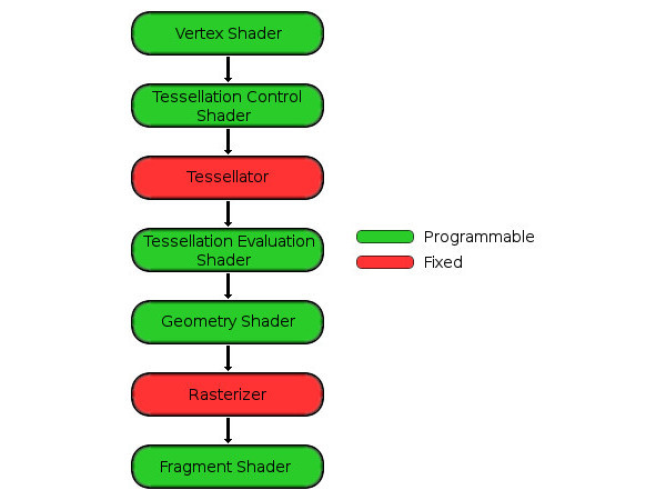
Having said all the above, it’s time to sum things up. Shaders are programs that run on the graphics hardware. In modern graphics APIs, they are obligatory parts of the graphics pipeline (the fixed pipeline is no longer supported). Every pixel drawn to the screen must be processed by shaders, no matter how lame or cool it is. Some shader types are optional and can be skipped, but not all of them. How much processing is done in shaders and how much is done on the CPU is up to the developer to decide. One can have very simple shaders and do everything on the CPU. Another option is to split the load among the two. Or maybe do everything in shaders. While it’s up to the developer to decide, what the developer chooses will significantly affect the performance of the application. It might feel obvious that moving everything to shaders is the way to go, but it’s not always the case. At the end, it’s the CPU that knows what should be rendered, how and when, and it has to continuously communicate these to the GPU. They have to collaborate to produce the end results, and they heavily affect each other. It’s quite common to see performance bottlenecks caused by nothing but the communication overhead, while the CPU and the GPU are idle or not actually doing any constructive work. With background covered, it’s time to dive into more details.

The Graphics Pipeline

This is a simplified (parts were intentionally omitted) version of the OpenGL 4.4 pipeline. There are several other shaders besides the vertex and fragment shaders. Don’t worry, we won’t have to deal with them now! OpenGL is mainly for desktop operating systems. What we are interested in is OpenGL ES (for embedded systems). Here is a simplified version of the OpenGL ES pipeline,

Much easier! When it was first introduced, mobile devices weren’t a match for desktop OpenGL, so another standard had to be written for limited configuration devices. OpenGL ES is for most a stripped down version of OpenGL. However, it does deviate from OpenGL at various places. Since WebGL is meant to be run in browsers, it has to be universal enough to work on both computers and mobile devices. Therefore, WebGL and OpenGL ES share a lot. WebGL 1.0 is based on and equivalent to OpenGL ES 2.0, and WebGL 2.0 is based on and equivalent to OpenGL ES 3.0. The shading language used in WebGL is the same as the one used in OpenGL ES. It’s called GLSL ES (OpenGL Shading Language). Hence, this is also the WebGL pipeline. As of the time of writing this article:

• Mobile devices grew much more capable. Now both desktop and mobile devices are converging towards using the same API, namely Vulkan.
• Experimental Vulkan drivers were shipped by nVidia, AMD and Intel for Windows and Linux desktop operating systems.
• MacOS is still stuck at OpenGL 4.1 (OpenGL 4.5 was released in 2014), and Apple shows no signs of implementing Vulkan on any of its devices. Instead, it’s focusing on its proprietary Metal API.
• The mobile market is dominated by OpenGL ES 2.0/3.0 devices (not even 3.1).
• WebGL 2.0 has just been released, and its support is still experimental in Chrome and Firefox. It’s not supported at all in Safari, Edge and Internet Explorer 11. Whether Vulkan will ever come to browsers is still unknown.

It’s quite reasonable to say that WebGL 1.0 (or even 2.0 if we are looking a little bit ahead) is still our best choice for maximum compatibility for years to come. WebGL is basically the only API that works on all major platforms. Lets get back to our WebGL pipeline.

Vertex Shader

To draw anything, it has to be made up from primitives. Primitives are made from vertices (points in 3D space) and faces joining these vertices (depending on the primitive in question). You can draw points, lines and triangles in WebGL. The most commonly used primitive is the triangle, so we’ll stick to it. However, the other primitives may become very handy depending on your application. The vertices enter the pipeline at the vertex shader. How the vertices are represented is totally up to you. For example, you may decide that each vertex needs to have an xy pair for position. If you are doing 3D then maybe xyz is more appropriate. You may decide that each vertex has a color, why not! Maybe a pair of texture coordinates, a normal vector and an id that represents what object it belongs to. You decide what works for your application. This is known as the Flexible Vertex Format (in DirectX terminology), or just vertex format (in OpenGL). Each one of these vertex parameters is referred to as an “Attribute”. Each and every vertex is then processed by the vertex shader you provide. What does the vertex shader do? How could I know! Again, it’s up to you to decide what it actually does. Typically it’s used to transform the vertices to their final locations on the screen. This includes accounting for their location with respect to the camera, any scaling or rotation needed and projecting them onto the viewing plane (typically the screen) using your desired projection (orthogonal, perspective, fish-eye …whatever). It can also be used to apply vertex animations. For example, waves on a water surface, or a flesh like organic movement. Don’t be overwhelmed. Things will gradually clear up as you work your way through this series. All you have to know for now is that the vertex shader accepts arbitrary vertex data (Vertex Attributes) and some data that are constant with respect to all the vertices being processed (Uniforms). It then performs some arbitrary computations on them to decide the final vertex position and produce new arbitrary data for the fragment shader to consume (known as Varyings).

Our First Shader

We’ll be filling the viewport with a nice colorful gradient that fades in and out with time. For this we need 4 vertices (one for each corner of the viewport) and two faces (triangles) to join them. We’ll be using this simple vertex shader: Yes, it looks like it’s written in C. For the most part, GLSL has C like syntax, but is not C. GLSL is OpenGL’s way of making sure shaders are portable enough to work on every OpenGL compatible hardware. The GLSL code is actually shipped with the applications, and is compiled at run-time to the target hardware instruction set. This way you don’t have to re-write your shaders to support every type of hardware in the market. However, you can still do that! GLSL compilers face a great challenge, which is to generate optimized programs very quickly from the source code at run-time. They often fail miserably! A scene with moderately complex shaders can take several seconds to compile the shaders only. This degrades the user experience considerably. For this reason, OpenGL allows you to query the binary formats supported by the hardware to load pre-compiled, pre-optimized shader programs. Large game engines do this. There’s no reason to favor one way over the other. We can take the best out of both worlds. We can include the GLSL source code together with some compiled binaries in our applications. If none of our pre-compiled binary formats is supported, we just fall back to compiling at run-time. Now lets take a closer look on our vertex shader, This is a declaration of a variable named vertexPosition. It’s:

• global, since it is declared in the global scope. It can be used outside the main function.
• an attribute, which means that its value is a part of the vertex data associated with each vertex.
• read-only. Attributes are inputs to the vertex shader. They cannot be modified.
• vec3. A vector with three floating point components.

Another variable declaration. vertexColor is:

• global, just like vertexPosition.
• a varying. It’s an output from the vertex shader, so its value should be computed and set by it.
• vec4. A vector with four floating point components.

The shader entry point. This function is called once for every vertex to be processed. Before the main is called, all the attributes are initialized to the corresponding data of the current vertex. It takes no arguments, and has no return values. The outcomes of the shader are passed to the next stages of the pipeline in “varyings” or special variables. Here’s one of such special variables. gl_Position is where the vertex shader should write the final vertex position. It’s:

• a vector with 4 floating point components.
• a built-in variable. We don’t need to declare it.
• in homogeneous coordinates. Not only it has x, y and z components, it also has aw component. This component is particularly useful in perspective correct texture mapping. This is out of the scope of this article. Meanwhile, we set w to 1.0.
• normalized. WebGL uses the coordinates (-1, -1) to represent the lower left corner of your viewport, and (1, 1) to represent the upper right corner. It’s the responsibility of the vertex shader to make sure all vertices are transformed from their local coordinate systems to the correct viewport coordinates. Anything outside the viewport dimensions is skipped and is not drawn altogether.

It is also used by the later stages of the pipeline to do:

• Primitive assembly (like creating faces from vertices).
• Clipping (breaking faces that extend outside the clipping volume into smaller ones, and skipping the ones outside altogether).
• Culling (skipping faces that won’t be drawn because they are hidden by other primitives, or just facing backwards if we are drawing single-sided polygons).
• Any other fixed function operations needed by the pipeline.

Back to our important line, vec4 is called a vector constructor. It constructs a vector with 4 floating point components from the given parameters. In this particular case, it uses the 3 values of vertexPosition (which is a vec3) as xyz, and uses 1.0 for the w component. We could have also written: which has the same effect. We can also do this: Useless in this particular situation, but possible. Now check this one out: Interesting, huh? Yes, we can do that. We can even shuffle the order of the components, This is called swizzling. It comes at no cost, so use it! We can also replicate components, That’s not all! Since vectors are not always used as positions, you get to use different names to refer to your components, where rgba is usually used when referring to colors, xyzw for positions and stpq for texture coordinates. I’m not done yet! There’s more, GLSL ES is type-safe. It doesn’t allow implicit conversions between types. Thus, a vec3 can’t be assigned to a vec2. But applying the vec2() constructor to vertexPosition stripped it from its z component, turning it into a vec2. Therefore, the above lines work perfectly. Note: while GLSL ES doesn’t normally allow implicit conversions, there’s an extension to support it. So if it works on your hardware, don’t be too happy. It could break on other hardware. Welcome to the wildest nightmares of graphics developers! It often pays off to stick to the standard and make no assumptions. One last trick, Using vector constructors on a single scalar value replicates the value over all the components of the vector. vec4(1.0) is identical to vec4(1.0, 1.0, 1.0, 1.0). All the above forms do essentially the same thing, but some are more efficient than the others in this particular situation. You don’t have to maintain the lifetime of the resulting vectors. Consider them temporary, or registers. You don’t have to delete these when you are done using them. Moving on to the next line, Lets assume it wasn’t written like this. Instead, Remember when we said that gl_Position should be normalized, and that the viewport coordinates in OpenGL range from (-1, -1) to (1, 1)? In this line, we give the vertex a color based on its final location in the viewport. But color values are clamped to the range from 0 (darkest) to 1 (brightest). This means that values less than 0 are treated like a 0, while values above 1 are treated like 1. Since our viewport position ranges from -1 to 1, it means that any vertices in the negative area will be zeroed. What we want is to stretch the colored area over the entire viewport. Lets do this then: Instead of ranging from -1 to 1, the new range is from 0 to 2. We fixed the negative range problem, but we introduced another range in which all values are 1s. We want a smooth change everywhere on the viewport, so lets give the line its final look, Thus it ranges from 0 to 1. Exactly what we want! But this is not how we wrote it in the original program. What we wrote was: We just applied the division to the parentheses, nothing more. So what’s special about it? In this form, the line became a MAD instruction (Multiply then Add). Most hardware have MAD instructions, so executing this line takes one cycle instead of two. It gives twice the performance, and the code is not any less readable. Sure, the compilers should be smart enough to do this on their own, but you can’t guarantee that. Lots of low quality drivers get shipped every now and then! Note that, we are multiplying a vec4 by 0.5, then adding 0.5 to it. We are mixing scalers and vectors! Ehm, GLSL ES is type-safe and doesn’t allow implicit conversions during assignments, but operations among scalars and vectors are allowed. This is equivalent to: While this has the desired effect on our red and green components, it leaves the blue component in a different state. The red and green components are based on the vertex xy coordinates which range from -1 to 1, while the blue is based on the z coordinate, which is a flat zero over the entire viewport. Thus, multiplying by half and adding half results in blue being half over all the viewport. We’ll consider this a feature rather than a bug and leave it the way it is! We could have fixed it easily though (do it in your mind as an exercise). Phew! This concludes our first vertex shader! It just:

• appends a 1.0 to the vertex position attribute and passes it without modification to the next steps.
• assigns a color to every vertex by defining and using the varying vertexColor.

Lets move further down the pipeline and see what happens next.

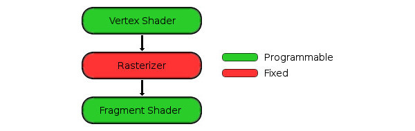
The Rasterizer

We’ve mentioned that there several fixed functions performed using gl_Position after the vertex shader, like primitive assembly, clipping and culling. The rasterizer comes after all such fixed functions. Its purpose is to rasterize the primitives created in the primitive assembly step. That is, turn them into fragments, which in turn turn into pixels. A fragment is a set of data contributing to the computation of a pixel’s final value. Setting a pixel’s final value needs one or more fragments, depending on your scene, your shaders and your settings.

Fragment Shader

Just like the way a vertex shader processes vertices one by one, fragment shaders process fragments one by one. Your powers of observation continue to serve you well! Yes, fragment shaders use GLSL as well, but they:

• don’t accept attributes, since they don’t process vertices.
• have a different set of input and output built-in variables. For example, they have no access for gl_Position (again, because they don’t process vertices), but they have access to another variable called gl_FragCoords, representing the pixel’s 2D position in the viewport, in pixels.

Moving on, We finally meet uniform variables! Uniforms are:

• accessible from both the vertex and fragment shaders, as long as they are explicitly declared in each.
• constant with respect to all vertices and fragments within a single draw-call (we get to know what a draw call is in the following article. For now, their values are set by the CPU and are not per-vertex or per-fragment).
• just like regular constants, using them for branching (conditionals and loops), texture look-ups (reading from textures) or dereferencing arrays can speed up things a lot. It’s because the hardware knows that their values won’t change throughout the pipeline, so it can perform look-aheads, prefetches and predict branching.

It’s also the first time we meet precision qualifiers. GLSL ES support 3 types of precision qualifiers that apply to integers and floats:

• lowp. Low Precision. That’s somewhere between 9 and 32 bits worth of precision. Floats of this type can hold values in the range [-2, 2], and are accurate to steps of 1/256.
• mediump. Medium Precision. Somewhere between 14 and 32 bits worth of precision, but at least as precise as lowp if lowp is within this range. Floats of this type can hold values in the range [-2¹⁴ , 2¹⁴].
• highp. High Precision. 32 bits worth of precision (1 sign, 8 exponent and 23 fraction). Floats of this type can hold values in the range [-2¹²⁶, 2¹²⁷]. However, implementing this precision is not mandatory. If the hardware doesn’t support it, it is reduced to amediump.

GLSL hardware is allowed to ignore all precision qualifiers and treat everything as highp if it wants. It is also allowed to choose any precisions within the supported ranges. WebGL allows you to query your device to get the exact specification of the implemented precision types. Giving your variables appropriate precision qualifiers affects performance and compatibility significantly. Always use the lowest precision level acceptable. For example, for representing colors, lowp is the way to go. Since only 8 bits are used to represent every color component in “true color” configurations, lowp is more than enough. Unless of course, you are doing some fancy stuff, like HDR (High Dynamic Range) and Bloom effects. Back to our line, This line declares time to be a float uniform of mediump precision. In GLSL ES fragment shaders, specifying precision when declaring variables is mandatory, unless we declare a global default: The above line instructs the compiler to treat all floats without a precision qualifier asmediumps. If so, we can write, We said that uniforms are accessible from both the vertex and fragment shaders, as long as they are explicitly declared in each of them. If that’s the case, they are required to have the same precision. They are required to appear the same to the shaders, and graphics hardware may even use the same storage for them in both the vertex and fragment shaders. Technicalities aside, we are going to update this uniform every frame, adding to it the time elapsed since the last frame in seconds. This will allow us to change pixel colors with time to achieve a nice fading in/out effect. To the next line, We have seen vertexColor declaration before in the vertex shader. But unlike uniforms, these are not the same! This vertexColor:

• is an input to the fragment shader, so it’s read-only.
• represents vertex color as seen by this particular fragment. Since this fragment belongs to the body of a primitive, it lies in the distance between a number of vertices forming this primitive (unless it coincides with a vertex, or the primitive is a point).
• gets its value by distance-based smooth interpolation of the values of vertexColor set by the vertex shader at the vertices forming the primitive. The rasterizer is responsible for such interpolation.
• is not that same as the vertex shader vertexColor, so it doesn’t have to have the same precision qualifier.

That’s the use of varyings. They are arbitrary data produced by the vertex shader to be interpolated and consumed in the fragments. Lets carry on with our shader, Just like in the vertex shader, it’s the shader entry point. It’s called once for every fragment to be processed. Before the main is called, all the varyings are initialized to the corresponding data of the current fragment. It takes no arguments, and has no return values. The outcomes of the shader are passed to the next stages of the pipeline in special variables. gl_FragColor is one of such special variables. It’s where the shader writes the final value of the fragment, if there’s only one color buffer attached. The fragment shader can write to multiple buffers at the same time, but this is beyond the scope of this article. There’s something interesting about fragment shaders in which they differ to vertex shaders. Fragment shaders are optional. Not having a fragment shader doesn’t make the pipeline useless. There are reasons why you might want to disable fragment shaders altogether. One of such reasons is, if the only purpose of drawing is to obtain the depth buffer of the scene, which can used in drawing later to compute shadows. Also, fragment shaders can be used to do more than just set colors. They can alter a fragment’s depth, or maybe discard it altogether (although not recommended as this prevents hidden surface removal optimizations). They can also be one step of several steps before reaching the final results. So what’s written to gl_FragColor may not be a color at all. Finally, writing a value togl_FragColor doesn’t mean that it will find its way to the color buffer directly. There are still more stages in the pipeline that follow fragment shading. Stuff like blending (like when primitives are partially transparent), scissoring (discarding all fragments outside a certain rectangular boundary) or anti-aliasing (removing stair-like artifacts at the primitive edges). For example, when MSAA (Multi-Sampling Anti-Aliasing) is enabled, fragments don’t correspond to pixels directly. MSAA basically means that every pixel is sampled at slightly different locations and the result is the weighted sum of all the samples. In such case, a fragment only represents one sample among others contributing to the final looks of the pixel. Just like you can enable or disable anti-aliasing altogether, you can do the same with respect to scissoring and blending. There’s an extension that allows you to read from the target buffer before writing to it in the fragment shader (which is called framebuffer fetching). It allows you to apply your own blend functions, or post-processing effects (like making everything in grey-scale) without having to render to an intermediate framebuffer. This is more powerful than the fixed blend modes, and makes the following blending step useless. In reality, sometimes the fixed functions are not physically present at all. Instead of implementing them in hardware, the driver appends their equivalent of shader code to your shaders without ever telling you. Returning to the line in question, Don’t be intimidated. It’s very easy. We want the gradient to fade out and in slightly, as if it’s breathing deeply. Lets do this step by step, Introducing our first built-in function, sin. It’s what you expect, the sine of an angle (trigonometry and stuff). It’s an oscillating function, as its value oscillates from 1 to -1 as the angle increases. This is what we need for our smooth fade in/out effect. However, the sine function goes all the way down, then spends half its time as a negative value before becoming positive again. All we want is a slight change in the color value, fading out about half the value then restoring it again. Lets do this, That’s more like it. The base value around which the color oscillates is 75% of the originalvertexColor. The color then goes down 25%, returns back then rises up 25% as the sine oscillates from -1 to 1. Perfect! No, not really perfect. While it works, there’s something important that we need to consider. Not all hardware supports vector operations (this comes as a shock, but unfortunately is true). Instead of performing vector operations in on clock cycle, they have to perform the operations one component at a time. Now take a look at the line we’ve just written, It performs vertexColor*0.25 first then multiplies the result by sin(time). This means, that all the components of vertexColor will be multiplied by 0.25 first, just to be multiplied by sin(time) again. That’s a total of 8 multiplications. Now consider re-ordering the parentheses, Now the 0.25 is multiplied by sin(time) before being applied to vertexColor. That’s a scaler by scaler multiplication (1 cycle). This reduces the number of multiplications from 8 to 5. A significant boost specially for hardware that doesn’t support vector operations. So as a rule of thumb, mind the order of your operations. Also, mask any components you are not using (like the blue component in our vertex shader). It can’t harm a good GPU, but can very well increase the performance of weak ones. One last rule. Use the built-in functions whenever possible. They are likely to be implemented in hardware and would be much better faster than your software counterparts. This concludes our vertex and fragment shaders pair. Since the vertex shader is tightly tied to the type vertex data provided, we’ll delay messing around with our vertex shader till later where we’ll address how to specify these data. For now, test and play around with the fragment shader as you please.

Finally that we have our working vertex and fragment shaders, lets do some analysis. This scene has exactly four vertices. This means that the vertex shader is called 4 times only every frame. At the same time, our fragment shader is being called once for every pixel on the viewport. Depending on its size, it could be thousands or even millions of times. This means that our fading in/out calculations are being performed too often, even though they don’t do anything pixel specific. We could move this calculation from the fragment shader to the vertex shader (just apply it to vertexColor there). As simple as this act is, it saves tons of computations and has the exact same result. So always double check if your computations really belong to the fragment shader or they can just be moved to the vertex shader. Looking further, we can see the parallel nature of shaders clearly. The exact same code is being executed over and over again on different inputs. There’s no reason why we should wait for the first batch of vertices or fragments to be processed before starting on the next one. That’s why graphics hardware is known to have massive numbers of cores. It’s because of the parallel nature of the pipeline steps that such numbers of cores can work together to finish the work load more efficiently. Another thing to notice is the pipeline nature. Every step can be performed immediately after the previous step finishes a simple task. For example, fragment shaders can start working right after the first primitives are assembled. The entire pipeline should always be in a state of motion, taking inputs and producing outputs, without having any stages idling. There was a time when vertex and fragment shaders had different capabilities, thus the number of vertex and pixel shader cores were fixed and stated in the hardware specs. In a scene like ours, it would be a total waste to have some vertex shader cores process 4 vertices then idle forever, while the fragment shaders are entrusted to a load thousands of times larger. Luckily, this is no longer the case. Vertex and fragment shaders evolved to become the same thing. This is known as the Unified Shader Model. The same cores are capable of acting as vertex or fragment shaders on demand. A scheduler is entrusted to monitor the workload and to balance the resources assigned to every stage to achieve maximum performance. Such flexibility unlocks new horizons for computing on graphics hardware. Shader cores are now used to perform not only graphics, but other parallel natured compute intensive applications. But don’t jump onto the wrong conclusion. While the cores could be the same, the resources available to different stages of the pipeline still differ. So not everything you can write in a vertex shader can be done in a fragment shader, and vice versa.

Conclusion

There is a lot more that could have gone into this article, but that’s enough to get you started. Next in this series, we cover how to initialize and use shaders in your WebGL applications using JavaScript. I hope this was helpful. Thanks a lot for reading!

References and More Reading

• The history of graphics hardware
• History of programmability in OpenGL
• OpenGL rendering pipeline overview
• WebGL 1.0 quick reference card
• GLSL optimizations
• Apple OpenGL ES best practices